Key takeaways

• The policy world is engaged in an ongoing debate about the extent to which economic policy should be “place-based”. Should economic policy target programs for poor people or programs for poor places?
  
• One argument in favor of “place-based” policy (PBP) is that policies may be more cost-effective in some places than in others. For example, a jobs program could be more effective in a region with persistently low employment rates than in an area with high employment rates.
  
• A new framework for evaluating the effects of public policy, the “Marginal Value of Public Funds” (MVPF), makes it easier to compare policies’ effects across different studies.
  
• We generate a series of 66 “geographic” MVPFs that can be tied to a specific place and time.
  
• We do not see any relationship between the MVPF observed in these studies and underlying geographic economic variables, including the unemployment rate or the elasticity of employment. We are unable to rule out the possibility of very strong positive or negative relationships.
  
• This suggests that further research may be needed to determine whether place-based policies are appropriate. Additionally, policy efforts should aim to deliberately generate more data by varying the locations that receive place-based policy funding.

Introduction

Economists have typically been critical of place-based policies (PBPs), preferring to provide economic support to people directly. This has been justified by the flexibility of the U.S. labor market—if a person is unemployed or underpaid, they could simply move to an area with higher labor demand. At worst, they could simply wait out local economic shocks. As such, policymakers should direct their attention to “people, not places.”¹

In recent years, this belief has begun to shift. First, it’s become apparent that residency is more “sticky” than economists once believed.² A person who loses their job for whatever reason (for example, shocks related to automation or international trade) is likely to stay in the same area they were born in and have family and other networks. Moreover, negative shocks to a location tend to be more permanent than was previously assumed. High unemployment in a small geographic area at an earlier time predicts high unemployment decades later.

 In theory, this suggests a new role for place-based policies. If people are unable or unwilling to move, policymakers should consider policies explicitly targeted at increasing incomes in low-opportunity areas. A 2018 Brookings study by Benjamin Austin, Edward Glaeser, and Larry Summers suggested that pro-employment policies (such as an enhanced Earned Income Tax Credit) could be targeted at low-employment areas to induce employment and increase welfare.³

Policymakers have taken this shift to heart, and place-based policy has been a centerpiece of the Biden administration.⁴ Brookings estimates that the 117th Congress has funded 18 place-based programs, totaling over $80 billion in spending.⁵ Even Donald Trump’s proposed “Freedom Cities” initiative could be considered a place-based policy.⁶

There is a great deal of theoretical evidence in favor of place-based policy⁷ but limited empirical evidence. There are at least two challenges. First, a place-based policy is, by definition, targeted at struggling regions. If a region continues to struggle after the PBP is initiated, is that evidence that the policy was ineffective or that more needed to be spent? If the region is thriving, does that suggest that the policy worked or that the region was going to prosper no matter what? The targeting of programs in itself makes it hard to assess what worked.

Second, so far, most place-based policies have been hard to compare because many of them are one-off interventions. How do you compare the effect of a “place-based” grant to locate a semiconductor facility in an area with few high-tech jobs to a highway repair bill? How do you compare a workforce development program aimed at people without college degrees to a public housing development?

Conventional cost-benefit analysis struggles with these issues. While individual papers may provide estimates of cost-benefit analyses, the frameworks and assumptions used vary across papers and disciplines, making it difficult to assess the differences among programs.

Marginal Value of Public Funds

Recently, economists Nathaniel Hendren and Ben Sprung-Keyser have proposed a method for estimating the Marginal Value of Public Funds (or MVPF) across a large variety of programs.⁸ They argue that MVPF analysis allows for a more broadly transferable estimate of the benefits of a program relative to the costs.

The MVPF is simply the ratio of a program’s beneficiaries’ “willingness to pay” for their benefits divided by the program’s net fiscal cost to the government. 

“Willingness to pay” means “How much would someone pay to receive the program?” While conceptually it’s possible to measure this directly (for example, by auctioning off program slots), this rarely happens in practice. Most MVPF analyses instead measure the economic benefits of a program and then convert to a “willingness to pay” estimate. For example, if a program increases wages by $2,000, you would estimate the “net present value” (how much that future increase is worth to you today) of the wage increase by applying a discount factor (typically 3%) to each subsequent year. If a program increased longevity by one year, that could be multiplied by the “statistical value of a life’ calculated by government agencies.

“Net fiscal cost”, in this context, accounts for two things—both the upfront cost of the program itself (how much it cost the government to run the program) and any subsequent downstream changes in government spending or revenues. For example, a program that increased beneficiaries’ income would also increase the government’s tax revenues.

MVPF differs from traditional benefit-cost ratio (BCR) analysis in two ways. First, instead of subtracting the change in revenues from the denominator, BCR adds it to the numerator. Second, in BCR both the “Upfront Cost” and “Change in Revenues” values are multiplied by an estimated “Welfare Cost of Taxation” (ie, the economic drag caused by the necessity of increased taxes to pay for a given program). The “Welfare Cost of Taxation” variable is particularly important, because economists do not consistently agree on the value of that number, or how to best assess it. This adds a bit of wiggle room that makes it difficult to compare one value to another.

There is an ongoing discussion about which of these formulas is best for policy analysis.⁹ Regardless, a key advantage of the MVPF is that it is easier to derive an MVPF from a causal analysis, such as a randomized trial with a treatment and control.¹⁰ You no longer need to estimate the welfare cost of taxes (which differs from economist to economist for somewhat arbitrary reasons), and the concept of willingness to pay divided by net total cost is easier to conceptually link to a given impactestimates. As such, the MVPF can be used as a unifying framework to estimate the value of a wide range of studies from different domains.

In this paper, we set out to build a database of MVPFs across geographic areas. We do this by looking at the MVPFs already assembled at the Policy Impacts Library,¹¹ determining whether a given MVPF is attached to a particular geography, and, when possible, deriving novel geographic MVPFs (for example, if a particular intervention was attempted in multiple areas Policy Impact Library would only include a single MVPF, but you could calculate a separate MVPF for each location). We then compare the calculated MVPFs to two important variables of local labor market health — the unemployment rate and the “elasticity of employment” — a measure first introduced by Austin, Glaeser, and Summers that estimates how much an area’s employment level responds to increased incentives to work.¹² 

The paper is organized as follows: we begin with a high level summary of our conclusions. The next section gives a high-level overview of the findings, briefly summarizing them for an interested policy audience. 

The subsequent sections provide details on the data. First, we look at the full data set across all policy areas. We then break out the data by specific policy areas that have large samples (the effect college on children,¹³ housing, and workforce development). Next, we look at individual studies where we are able to calculate unique MVPFs in different locations. We then examine subcomponents of the MVPF itself to see how changes in geography affect costs and benefits separately.

Finally, an appendix gives details on the calculation of geographic MVPFs in the papers where we had to assemble a novel MVPF.

Key findings

• There are not enough geographic MVPFs to draw firm conclusions. When we started this project, it was unclear how many MVPF studies would have a geographic component. After going through the Policy Impacts Library, we found 63 MVPFs that we associated with a specific location. Most of these were from papers that measured the effects of a policy change within a single state. We also found seven papers with multiple geographic MVPFs, either calculated in the original paper or decomposed from other results.
  
  Sixty-three estimates are a limited sample; while we report on the findings and some results are suggestive, any firm conclusions will have to wait for more data.
  
• Less than half of U.S. states have an MVPF study associated with them. Only 21 U.S. states could be associated with a MVPF. Three states — New York, California, and Texas — are responsible for more than 40 percent of the total sample of MVPFs. In addition to more studies in general, there needs to be a wider dispersion of studies across different states to better estimate the effects of different geographic locations on the MVPF. In particular, having more estimates from high-employment-elasticity states, such as Arkansas, Mississippi, Kentucky, and West Virginia, would be helpful. This is especially the case for RCT evaluations run across multiple states.
  
• There is substantial heterogeneity in how MVPFs are calculated. While calculating the MVPF for a given study may seem straightforward, there are substantial differences in how each study approaches the calculation. Most notably, older studies can observe the impact over a lifetime, while more recent studies cannot. Similarly, some studies are well set up to observe parts of the net fiscal cost of a program (for example, by recording participation in the Supplemental Nutrition Assistance Program). Others are not — and one would have to engage in a costly and time-consuming data merging process to collect it. As such, while the MVPF is theoretically a good measure for comparison across studies, in practice the necessary data is not always available.
  
• We cannot rule out very large effects of geography on MVPF – positive or negative. When estimating the effects of geography on MVPFs, we cannot draw firm conclusions. Moving from a low employment elasticity area (such as Wyoming) to a high one (such as West Virginia) could decrease the MVPF of an intervention by 17 percentage points or increase it by 14 — a wide range.
  
• It is possible that costs increase in high-elasticity areas faster than benefits. Place-based policy often starts by considering how the benefits of a policy could vary by area, but it is also possible for costs to vary. While we do not find a statistically significant relationship between either the costs or benefits and the elasticity of employment, the relationship for costs is somewhat stronger. This could suggest that place-based policy is more difficult than it was previously thought.
  

Main results

Data collection

Geographic MVPFs were calculated using the data from the Policy Impacts Library.¹⁴ For a complete discussion of how MVPFs were calculated, see the Appendix. Figure 1 provides an overview. Of the 133 MVPFs available in the MVPF library, we examined 89 (we excluded the “Criminal Justice” and “Social Insurance” sections since interventions in those sections were not well-tied to place-based policy). From those 89 papers, we assembled a list of 63 geographic MVPFs.

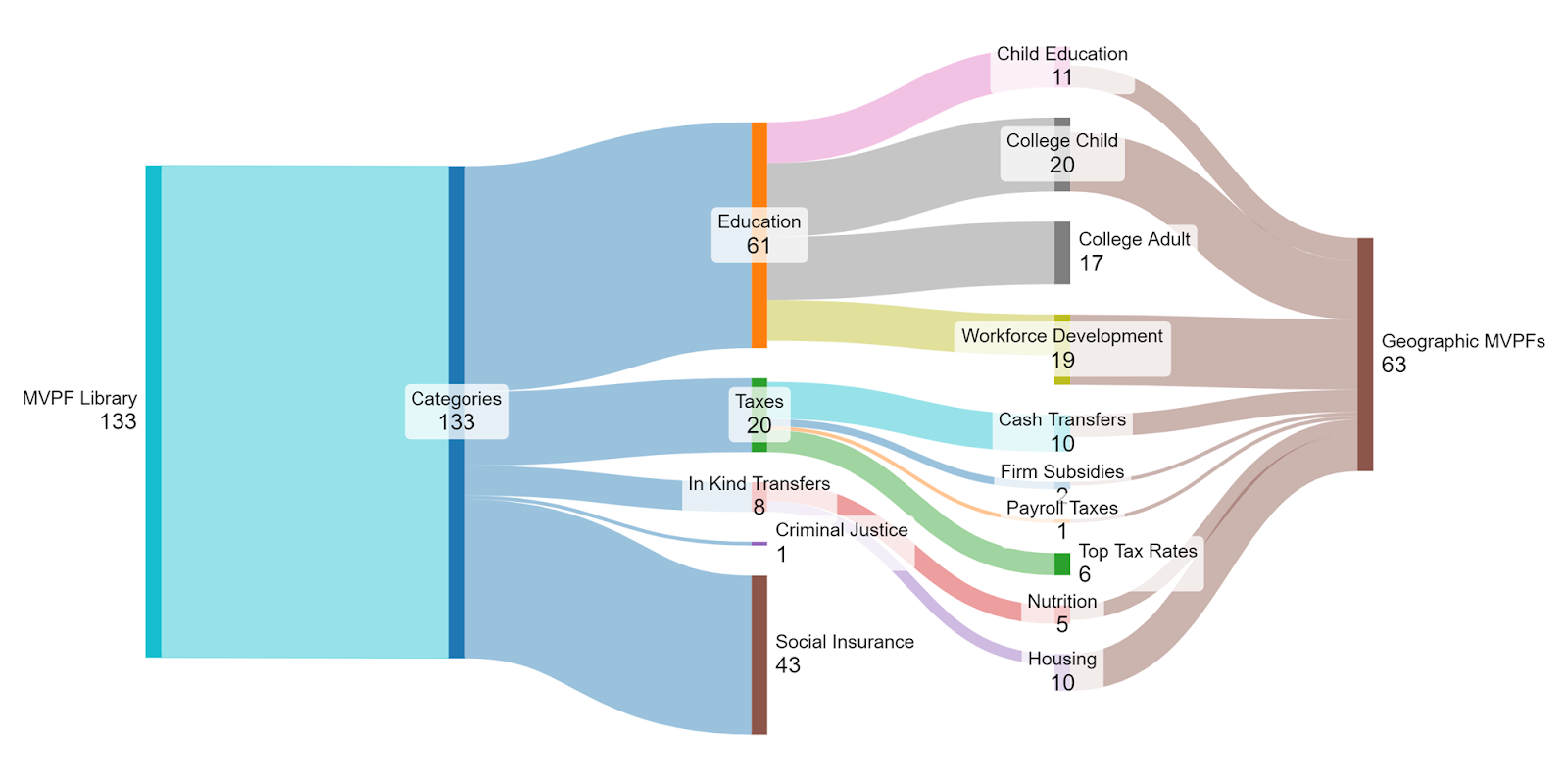Figure 1 – MVPF Sankey chart

There is not a one-to-one correspondence between geographic MVPFs and the MVPFs in the policy library. Many papers have MVPFs that are not tied to a sufficiently small geographic entity (for example, papers that calculated the MVPF for a policy that applies to the entire United States). Other papers examined a policy change within a single geographic area, allowing us to link that MVPF to a specific geographic entity. Finally, some papers had different results for different locations. While the MVPF reported in the Policy Impact Library was the MVPF for the pooled data, we were, in several cases, able to decompose the national MVPF into several local MVPFs.

A limitation of the MVPF data is that we only have geographic MVPFs for 21 states. The number of MVPFs observed in each state is partially driven by population size. Only three states have five or more MVPFs observed: New York, California, and Texas (the fourth, first, and second largest states). 

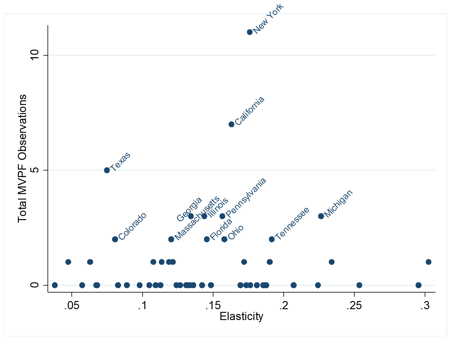
Figure 4 – Total MVPFs observed by state

There is no relationship between the number of MVPFs observed and the elasticity of employment. Dividing all states into three population-weighted terciles, we count 15 MVPFs for the tercile with the lowest elasticity of employment, 20 for the middle tercile, and 20 for the tercile with the highest elasticity of employment.

To assess the relationship between MVPFs and geographic areas, we focus on two economic measures: the elasticity of employment and the unemployment rate. These are both metrics that tell us about labor market slack in a region, which would conceptually mean that spending would be more likely to have an effect (at least through labor market channels).

The elasticity of employment measures how the employment level for prime-age men within a state reacts to shifts in labor demand. Austin, Glaeser, and Summers (2018) report the elasticity of employment for three states: Massachusetts, West Virginia (the state with the highest elasticity), and Wyoming (the state with the lowest elasticity). We replicated their work and report elasticities for all states in Figure 2 below.

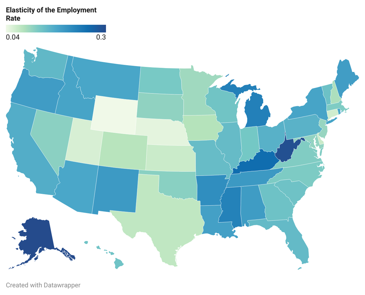
Figure 2 – Elasticity of employment, by state

The elasticity of employment is an estimate of how the marginal dollar spent subsidizing jobs would shift the employment rate among prime-age men. In states like Wyoming, where the employment rate is generally high, additional subsidies would have a limited effect. In states like West Virginia, where the employment rate is typically low, subsidizing labor demand could increase the employment rate substantially. 

The elasticity of employment has two weaknesses as used for our purposes. First, our estimates are only at the state level, using the Austin-Glaeser-Summers approach. That means that we do not have estimates for other geographic entities, such as cities, “rural” vs. “urban” areas, or non-U.S. entities. Second, the elasticity of employment is calculated using data from the 1980s through the 2010s. While Austin-Glaeser-Summers argue that the elasticity of employment is stable over the 1980-2010 period, it seems unlikely that this holds over more extended periods. As such, the elasticity of employment is not appropriate for MVPFs calculated from data that substantially precedes the 1980s. 

Because of these weaknesses, we also examine the relationship between geographic MVPFs and the unemployment rate. The unemployment rate can be readily obtained in more areas and over a longer period of time and is calculated in a fairly standardized manner internationally.

We examine the relationship between geographic MVPF and these two variables in multiple ways. First, we look at the entire database for a full data analysis. Next, we break down the relationship within particular subcategories, followed by specific studies. We then look at the components of the MVPF – the willingness to pay, the upfront cost of the intervention, and the net fiscal cost.

Full data analysis

Figure 3 shows the geographic MVPFs against the elasticity of the employment rate in the state in which the MVPF was recorded.

Because the MVPF is a ratio, some MVPFs can be very large. In cases where the program had a zero or negative net fiscal cost (i.e., cases in which the intervention pays for itself), the MVPF will be infinite. We have bounded the graphed MVPFs between 0 and 5 to make the graphs legible. In cases where the MVPF is less than zero (i.e., the intervention causes net harm to recipients), we plot the value at zero. In cases where the MVPF is five or more (the highest finite MVPF in our data set is 349), we plot the data at 5. An additional line above the 5 indicates studies for which the MVPF is infinite.

Figure 3 – MVPFs by elasticity of employment

There is no clear relationship between the magnitude of geographic MVPFs and the elasticity of employment on visual inspection. Because of the presence of infinite MVPFs, it is not possible to run a regression on the full data. One option is to winsorize the data by setting all data points above the 85th percentile or below the 15th percentile to the 85th and 15th percentile, respectively. If we do this, we observe a negative, non-significant relationship between the MVPF and the elasticity of unemployment. However, we cannot rule out either very strong negative or very strong positive relationships – the 95th percentile confidence interval ranges from -69.7 to 56.4.

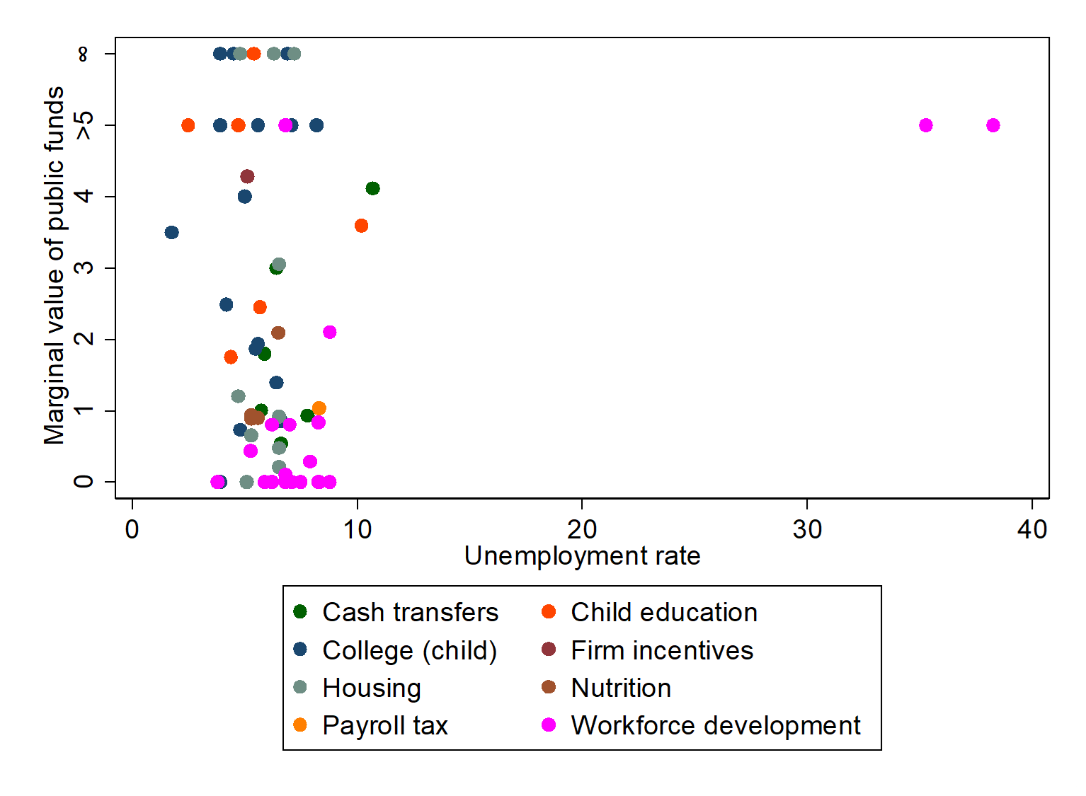
Figure 5 – MVPFs by unemployment rate

Figure 4 shows the MVPFs by the unemployment rate. The unemployment rate differs from the elasticity of employment graph in several ways. 1.) We can incorporate a broader set of geographic MVPFs by including MVPFs where we do not have elasticity estimates (this includes international MVPFs and Bastian 2023, which differentiates between “urban” and “rural” America 2.) While the elasticity of employment is a fixed variable for each state, the unemployment rate varies over time. We calculated the unemployment rate as the average unemployment rate in the state in the year(s) of the intervention(s).

The major visible difference between the elasticity and unemployment graphs is the two outlier workforce development observations with unemployment levels in the 1930s. These are observations from the Civilian Conservation Corps project during the Great Depression when the unemployment rate was very high. It is worth noting that the CCC MVPF is unique in that it includes the expected increase in longevity due to participation in the program. CCC participants lived approximately one year longer than non-participants, on average. The net present value of an additional year of life is substantial – it is more than half of the total willingness to pay for the CCC program. The CCC is the only program that has an estimate of the effects on longevity, as no other MVPF estimates are old enough to plausibly estimate such a value (the next oldest study is Abecedarian, with a 1972 start date).

Using the same winsorized data we used for the elasticity of employment, we can regress the unemployment rate on the MVPFs. Again, we see a negative, non-significant relationship but cannot rule out very strong negative or positive relationships – the 95th percent confidence interval ranges from -27.5 to 7.9.

Subcategory-level analysis

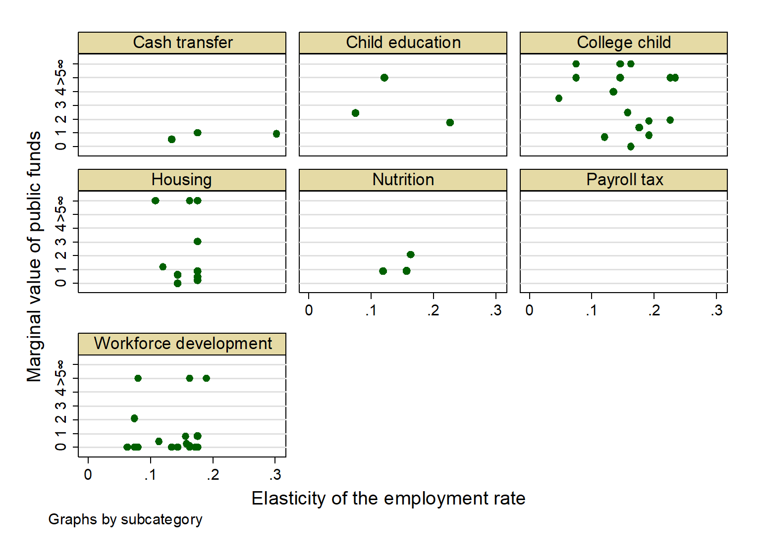
Figure 6 – MVPFs by elasticity of the employment rate, subcategory breakout

Figure 6 shows MVPF and elasticity of employment by MVPF category. We exclude “Firm Incentives” and “Payroll Tax” for this discussion. Both of those subcategories only have one observation, so we cannot analyze the relationship between geographic MVPFs and the elasticity of employment.

Similarly, “Cash Transfers,” “Child education,” and “Nutrition” each have only three geographic MVPFs. While we include graphs for each, this is insufficient observation for a subcategory analysis.

College child

We have 16 observations of geographic MVPFs within the “college child” subcategory.  This category refers to recent high school graduates who attended college (as opposed to adult learners). Fourteen observations come from individual studies with a single MVPF and two studies from different metrics for determining eligibility for the “Cal Grants” program. Nine of the geographic MVPFs are based on a regression discontinuity approach, where students were eligible for a scholarship if their GPA, SAT, income, or similar variable was above or below a specific threshold, allowing for an estimate of the causal effect. Other methodologies in this subcategory include differences-in-differences (2 studies), natural experiments (3 studies), panel data (1 study), and a randomized controlled trial (1 study). 

Within this subcategory, there is a wide range of MVPFs. Three geographic MVPFs (Pell Grants in Texas, Expanded Admissions to Florida International University, and Cal Grants using a GPA threshold) had an infinite value (i.e., the program would pay for itself when you account for the value of future taxes). One had a negative value (Cal Grants using an income threshold).

In the winsorized data, we observe a negative, non-significant relationship between MVPF and elasticity of employment within the “college child” subcategory, with a 95th percentile confidence interval of -166.5 to 121.2. We observe a positive, non-significant relationship between MVPF and unemployment rate with a 95th percentile confidence interval of -64.1 to 622.9.

Housing

Housing data comes from three studies: “Moving to Opportunity” (a five-site randomized trial), “Housing Vouchers in Chicago” (a single-site lottery program), and “NY 421 tax benefits”, a property tax exclusion for renting to low-income households. “NY 421 tax benefits” is unique in the data set in that the paper reports MVPFs at the neighborhood level—a far more granular level than any other paper. We report four MVPFs from this paper, the average MVPF for each quartile.

Again, we see a wide range of MVPFs, with three infinite MVPFs (3 Moving to Opportunity sites) and a single negative MVPF (another Moving to Opportunity site).

In the winsorized data, we observe a negative, non-significant relationship between MVPF and elasticity of employment within the “housing” subcategory, with a 95th percentile confidence interval of -538.4 to 345.6. We observe a positive, non-significant relationship between MVPF and unemployment rate with a 95th percentile confidence interval of -1181.2 to 1573.9

Workforce development

Workforce development data comes from three studies: the Civilian Conservation Corps evaluation (two sites), the Work Advance study (a four-site randomized trial), and the JOBSTART study (a 13-site randomized trial). We report 19 MVPFs in total.

The highest observed MVPF is a California JOBSTART trial, with a MVPF of 13.9. This is followed by the two Civilian Conservation Corps studies (6.1 for New Mexico and 5.4 for New Mexico). A second JOBSTART program from Texas has a MVPF of 2.1. All other MVPFs are below 1.

In the winsorized data, we observe a positive, non-significant relationship between MVPF and elasticity of employment within the “workforce development” subcategory, with a 95th percentile confidence interval of -27.4 to 39.4. 

We observe a positive and significant relationship between MVPF and the unemployment rate. The coefficient is 15.3, with a standard error of 3.2. This suggests that for every 10 percent increase in the unemployment rate, the MVPF increases by 1.5. The 95th percentile confidence interval ranges from 8.4 to 22.2.

This result is driven by the two Civilian Conservation Corps observations, which have both a high MVPF and a high unemployment rate. When they are dropped from the sample, the coefficient is no longer significant, and the 95th percent confidence interval ranges from -50 to 50.2

Individual studies analysis

Figure 7 shows the MVPFs plotted against the elasticity of the employment rate in 5 studies for which we have multiple MVPF values.

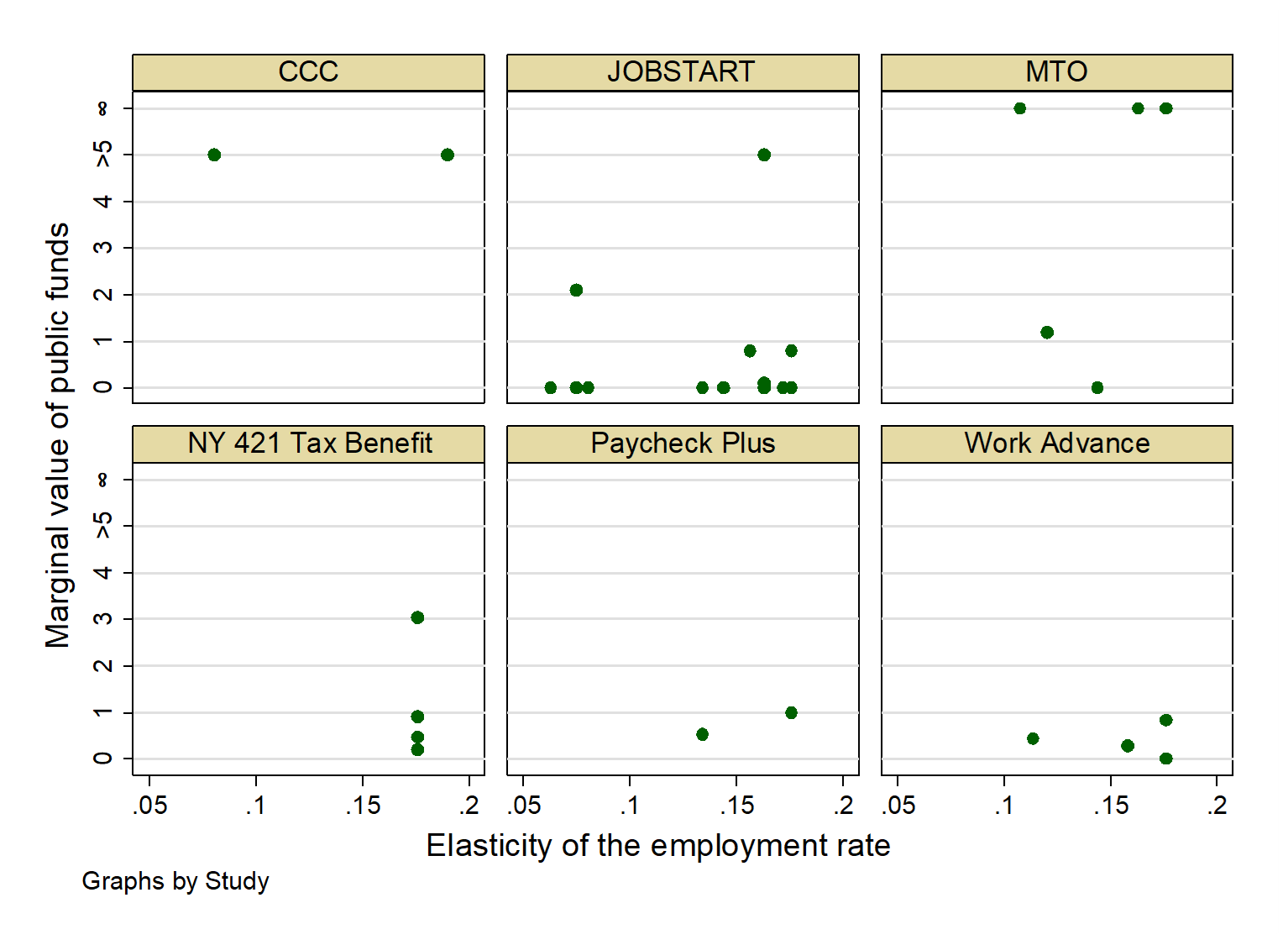
Figure 7 – MVPFs by elasticity of the employment rate, study breakout

• Civilian Conservation Corps – The Civilian Conservation Corps (CCC) study looked at the effects of employment in the CCC during the Great Depression. This study had two sites: New Mexico (MVPF 5.4) and Colorado (MVPF 6.1). While New Mexico has a higher elasticity of employment, given the time elapsed between the Great Depression and the calculation of elasticity, this is unlikely to be relevant. Both states had high unemployment rates during the 1930s, with New Mexico’s somewhat higher (38.3% versus 35.5%)
  
• Moving to Opportunity – The Moving to Opportunity study looked at the effects of a voucher that encouraged families in public housing to move to high-economic mobility areas. This randomized controlled trial (RCT) had five sites: Baltimore, Boston, Chicago, Los Angeles, and New York. There is a wide range of MVPFs. Three sites (Baltimore, Los Angeles, and New York) had an infinite MVF because the intervention paid for itself. The Boston site had an MVPF of 1.2, suggesting a Willingness to Pay that was 20% greater than the cost of the program. The Baltimore site had an MVPF of -3.2, as the treatment group’s income actually decreased.
  
• Paycheck Plus—The Paycheck Plus study looked at the effects of an Earned Income Tax Credit-like program for single individuals. This RCT had two sites: Atlanta and New York City. The Atlanta site had a somewhat lower MVPF (0.5) than the New York Site (1.0), largely because there was a decrease in working among Paycheck Plus recipients in the Atlanta site.
  
• Work Advance—The Work Advance study examined the impact of a training program that provided low-income individuals with occupational skills in high-demand areas. This RCT was tested in four sites: The Bronx (NYC), Brooklyn (NYC), Tulsa (OK), and Cleveland (OH). MVPFs ranged from 0 (Brooklyn) to 0.83 (the Bronx).
  
• JOBSTART – The JOBSTART study was a vocational training program modeled after Jobs Corps. This RCT was tested in 13 sites. The highest MVPF was 13.9 from the site in San Jose, California. JOBSTART recipients on that site saw an annual income increase of $6,715. The second-highest MVPF was 2.1 in Dallas, TX. All other MVPFs were less than 1. The lowest MVPF was -5.1 in Denver, CO.

MVPF components

The MVPF is the ratio between the willingness to pay for a program and the net fiscal cost (the upfront cost of the program as well as any changes to government revenues due to changes in tax receipts or spending). For the studies above, where we have multiple geographic MVPFs for a single program, we can look at the cost and benefits separately.

We can do this across studies by taking the z-score for each site. The z-score is the value for a given site within a study minus the average value, which is then divided by the standard deviation. Performing this calculation allows us to put all the studies on a similar approximate scale.

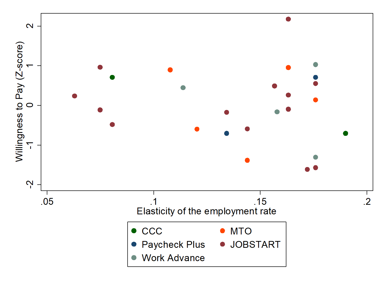
Figure 8 – Willingness to pay by elasticity of employment

Figure 8 shows the z-score of the willingness-to-pay variable for each of the five studies with multiple MVPFs against the elasticity of the employment rate. A regression shows that willingness-to-pay has a negative, non-significant relationship with the elasticity of the employment rate, with a 95% confidence interval ranging from -11.8 to 4.4.

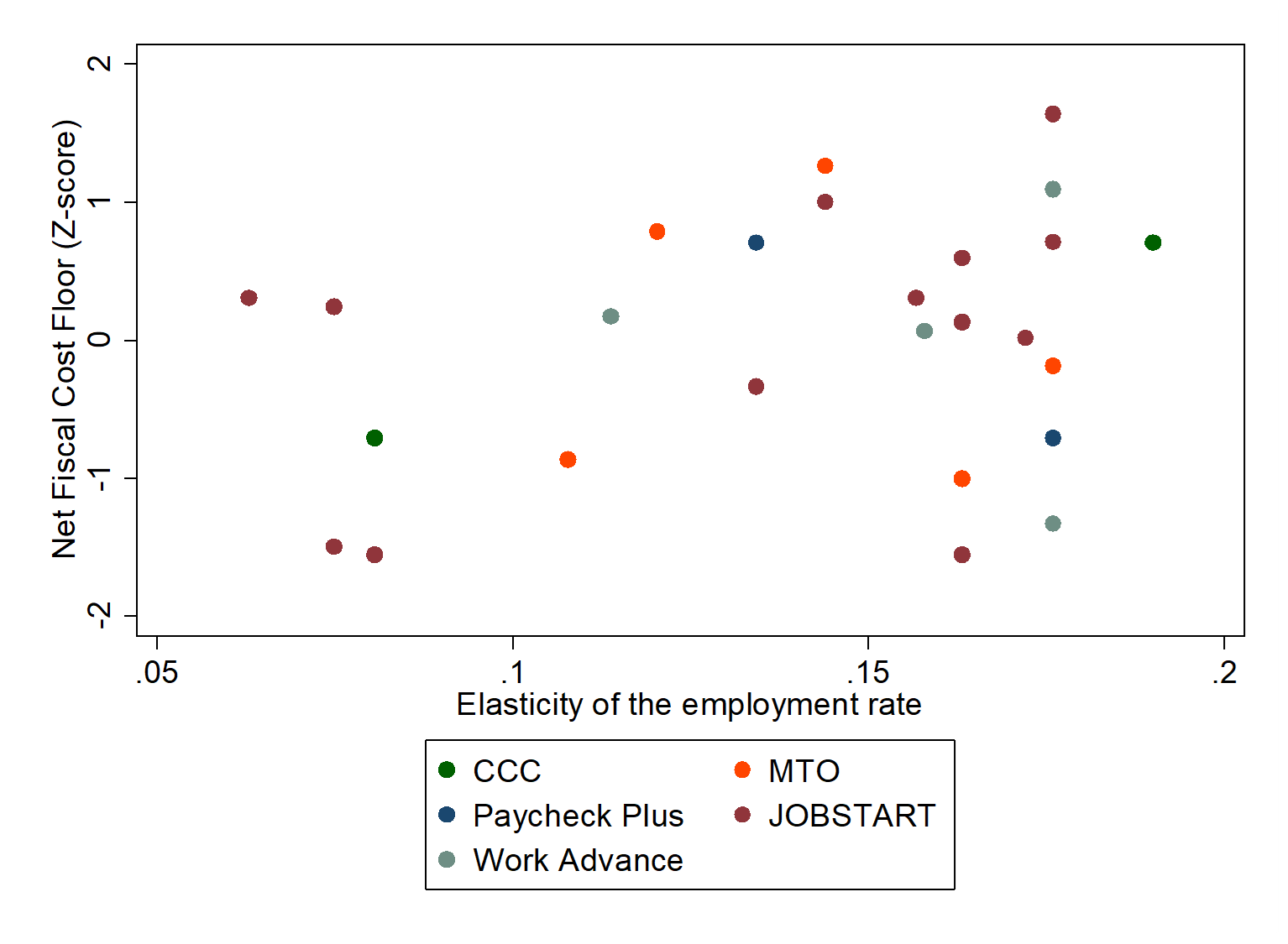
Figure 9 – Net fiscal cost by elasticity of employment

Figure 9 shows the z-score of the net fiscal cost variable for each of the five studies with multiple MVPFs against the elasticity of the employment rate. A regression shows that willingness-to-pay has a positive, non-significant relationship with the elasticity of the employment rate, with a 95% confidence interval ranging from -2.8 to 16.1.

While neither the “Willingness to Pay” nor “Net Fiscal Cost” variables are significant, it is intriguing that we see a stronger relationship between “Net Fiscal Cost” and elasticity of employment than “Willingness to Pay” and elasticity of employment. Elasticity of employment is a measure conceptually designed around anticipating areas that would have more program benefits. If it is instead the case that the fiscal costs of programs increase faster, that limits the potential for place-based policies.

Conclusion

The Marginal Value of Public Funds (MVPF) framework offers a promising tool to compare policy impacts across different locations. However, our initial research reveals that there is still much to learn about the relationship between geographical economic variables and policy effectiveness. The lack of a consistent correlation between geographic MVPFs and variables like the elasticity of employment and the unemployment rate suggests that further research is necessary to draw more definitive conclusions. In particular, we would like to see more MVPF estimates in high employment-elasticity states, which would give us a better understanding of whether those states generally have higher MVPFs. 

In addition, it would be valuable to have more multisite studies where the same treatment is tested within different areas. There is substantial heterogeneity of effects and MVPFs across sites, and these are under-discussed in the literature, which typically reports on the main effects of the treatment and only includes site heterogeneity effects in the appendix (if they are discussed at all). The treatments we examined in this report show a wide range of effects sizes and MVPFs. Helping policymakers anticipate where programs will get the most “bang for the buck” is essential.

As this field of study evolves, it will be crucial to integrate more robust and diversified data to better assess the true impact of place-based policies on economic health and community well-being.

Appendix I: MVPF construction

Overview

This section describes the methodology by which we arrived at the geographic Marginal Value of Public Funds (MVPFs) used for the analysis in the paper. We started by looking at the corpus of MVPF estimates available at the Policy Impacts Library at https://www.policyimpacts.org/policy-impacts-library. Some MVPF estimates do not apply to specific, small geographic areas, making them impractical for place-based policy analysis. In some cases, it is possible to decompose the aggregate MVPF in the Policy Impact Library into specific MVPFs for individual sites. For example, a randomized controlled trial of a workforce program may have been tried in multiple states. While the MVPF reported at the Policy Impact Library might be a national estimate, we can calculate or estimate each site’s individual MVPF if separate impact and cost data are available.

In many MVPF calculations, we simplify by assuming that the site-level cost or benefit components have a linear relationship with the aggregate MVPF data. For example, if the 2-year increase in tax revenues for one site was 10% higher than the national average, we treat the net present value (NPV) of future taxes as also 10% higher than the national average rather than estimating a separate net present value. This method substantially simplifies the calculations, especially for more complicated MVPF calculations that consider changes in lifespans or tax regimes over time.

As of March 2024, the Policy Impact Library included 133 MVPF estimates. These estimates are divided into six categories: “Criminal Justice”, “Education”, “In Kind Transfers”, “Social Insurance” and “Taxes”. For our analysis, we only examine three of these categories, “Education”, “In Kind Transfers” and “Taxes”, dropping “Criminal Justice” and “Social Insurance” as the former includes only a single study and the latter is only minimally connected to place-based policies. This leaves us with a set of 89 MVPF estimates.

We identified one or more geographic-specific MVPF estimates in 37 of these 89 papers. For our purposes, we define a geographic MVPF as an MVPF that applies to an entity smaller than the United States as a whole. These studies include MVPFs on sub-areas such as states or cities and MVPFs from nations smaller than the U.S. (this includes Israel, France, Nicaragua, Sweden, Tamil Nadu (an Indian state), and the United Kingdom).

A wide range of methods are used to estimate the impact of the relevant programs and, hence, the MVPF. Eight papers are purely descriptive estimates. Two papers use a differences-in-differences estimation. Three papers use a natural or policy estimate as a source of plausible exogenous variation. Two papers use panel-based fixed effects. Eleven papers are randomized controlled trials. There are eleven regression discontinuities and a single synthetic control paper. The diverse methodologies used across studies complicate direct comparisons of their strengths and limitations. In some cases, papers use changes in local tax incentives that apply to every person in a state over several years. In other randomized trials, a few hundred people receive treatment. The number of observations in Table 1 is based on the number that best corresponds to the treated group, but it cannot be used as a basis for comparison across studies, especially studies with different methodologies.

There are seven papers where it is possible to isolate multiple geographic MVPFs, ranging from papers with two MVPFs to papers with 14 MVPFs. These are generally papers in which a particular intervention was tested in various areas in a randomized controlled trial or where the researcher reported effects on multiple geographic subgroups.

In total, this gives us 63 individual MVPF calculations for particular geographies.

Figure A1 – Sankey chart of geographic MVPFs

We examine two variables to see if they are related to the MVPF. First, we use the state’s elasticity of the employment rate with respect to wages, as described in Austin, Glaeser, and Summers.¹⁵ This is an estimate of how male prime-age (25-54) employment within each state reacts to a change in the wage rate. We use the replication files from Austin, Glaeser, and Summers to create an index for each state.

Second, we examine the unemployment rate for each state or nation under consideration. The unemployment rate measures economic deprivation with a standard, international underlying concept that has been stable over time. That allows us to include international studies and older studies where male prime-age employment may not be readily available, such that we cannot use the Austin, Glaeser, and Summers estimate of employment elasticity.

The following section details our approach to deriving geographic MVPFs, focusing on novel estimates where previous literature or databases lacked specific calculations.

Derivation of geographic MVPFs

We calculated novel MVPF estimates for geographic entities in five papers where no such calculations appeared in the original paper or the Policy Impact Library summary. This section briefly describes the approach taken for each paper. We rely on the MVPF calculations in the original paper or the detailed walkthrough in Hendren and Sprung-Keyser¹⁶ to generate our estimates.

Civilian Conservation Corps

Aizer, Eli, Imbens, Lee, and Lleras-Muney estimate the impact of the Civilian Conservation Corps (CCC), a New Deal-era youth training program that hired young men to work in rural areas.¹⁷ They find that participation in the CCC has two major effects — an increase in the trainees’ wages and an increase in the trainees’ lifespan. The willingness to pay for the program increases as a function of the increased net present value of wages, and the fiscal externalities also grow as the participants will both pay for and receive more benefits due to their increased wages and lifespan. The MVPF calculations in the paper include both of these effects. Their data includes separate impact data for the Colorado and New Mexico programs, allowing us to estimate MVPFs for both locations separately.

Cost estimates

The upfront cost of the program was estimated to be $1,004 in 1939.¹⁸ There was no separate breakout of costs by geographic area, so we used this cost for Colorado and New Mexico.

One effect of CCC participation was increased longevity. CCC participants lived 0.013 log years longer than non-participants for each year of service, about equal to an additional year at age 70). In Appendix Table 8, Aizer et al. show that Colorado participants also increased by 0.013 log years per year of service, while New Mexico participants increased by 0.014. Given the imprecision of the reported difference and the small impact (the 0.001 difference in log years would result in one or two additional months of life), we default to using the national average instead of separately calculating the effects of differential increases in longevity.

We do look at the differential estimates in pay and Social Security benefits. Appendix Table 8 in Aizer et al. shows that Colorado participants saw their primary insurance amount (PIA – the monthly Social Security benefits) increase by $15.68, while New Mexico participants saw an increase of $19.20. We use this to calculate the negative fiscal externalities of Social Security payments \by dividing the Aizer et al. estimate by the national average PIA increase and then multiplying by the specific state value. The final value is higher for New Mexico participants ($2,809.18) than for Colorado participants ($2,293.37).

We must also adjust for the positive fiscal externality of additional Social Security taxes paid. Appendix Table 8 in Aizer et al. shows that the increase in Average Indexed Monthly Earnings (AIME) for Colorado participants was $49.69 versus $46.74 for New Mexico participants. Again, we use the MVPF estimates for the national average as a baseline for our calculations. Colorado participants paid an additional $6,903.08 in Social Security taxes, while New Mexico participants paid $6,493.77.

The original MVPF calculations also examine the effects of CCC participation on SSDI claims, SSDI claiming age, and age at retirement. These are not broken out for New Mexico and Colorado participants, so we use the national-level numbers. In addition, there is no estimate of the positive fiscal externalities from the goods produced by the CCC. Following Aizer et al., we assume no benefits to CCC from goods production, with the understanding that the MVPFs will be a floor value.

The final cost estimate is $8,059.37 for Colorado and $8,984.49 for New Mexico.

Willingness to pay estimates

A major component of willingness to pay is the NPV of the increased longevity of CCC participants. Aizer et al. estimate this value to be $25,456.40. Again, we do not estimate a separate value for longevity across the Colorado and New Mexico sites.

Another component is the increased earnings of CCC participants. We use the state AIME parameters discussed above to estimate that by dividing the national MVPF by the national AIME and multiplying by the state AIME. The NPV of earnings increased by $13,520.23 for the Colorado participants and $12,718.57 for the New Mexico participants.

Two variables used by Aizer et al., the real wage when enrolled and the loss of SSDI benefits, do not have a geographic breakout. We use the Aizer et al. values of $11,390.36 and -$910.61, respectively.

The final willingness to pay is $49,456.38 for Colorado and $48,654.72 for New Mexico.

MVPF estimates

The Colorado program had an MVPF of 6.14 ($49,456.38/$8,059.37), and the New Mexico program had an MVPF of 5.3 ($48,654.72/$8,984.49).

There is no standardized unemployment data for the period of this study. We use the 1933 unemployment estimates from Murray and Ring’s 1937 report for our tables.¹⁹

Work Advance

Work Advance is a workforce development program that provides unemployed adults with occupational skills training. From 2011-2013, Work Advance was tested in a randomized trial across four sites: The Bronx, Brooklyn, Tulsa, and Cleveland. The results of this RCT are reported in Hendra et al.²⁰ The MVPF is calculated in Hendren and Sprung-Keyser.²¹ Costs and impacts are reported separately for each site, allowing us to estimate a MVPF for each site individually.

Cost estimates

Program costs are listed separately in Hendra et al., Table 4.2. Program costs ranged from $5,203 to $6,666. In addition to program costs, Hendra et al. reported the reduction in out-of-program costs in Table 4.2 (i.e., people in the control group may have enrolled in other federally funded vocational programs). The average decrease in out-of-program costs ranged from -$244 to -$2,278 across sites.

Additionally, Hendren and Sprung-Keyser calculate the net present value of increased tax revenues from the Work Advance programs. This results in a -$11 cost, averaged across all sites. Prorating this by the two-year earnings increase across all four sites (available in Appendix Table A.7) gives us individual site estimates ranging from -$8.76 to $0.50.

In total, costs range from $5,868.50 to $3,467.24.

Willingness to pay estimates

Following Hendren and Sprung-Keyser, we use the NPV of future after-tax incomes to measure willingness to pay. Hendren and Sprung-Keyser estimate this to be $3,635 across all sites. We again prorate their estimate by each site’s individual two-year earnings increase reported in Hendra et al., giving us a range of WTP from -166.33 to $2,894.92.

MVPF estimates

Dividing the willingness to pay by the cost for each site gives us the MVPF, which ranges from -0.03 (the site in Brooklyn) to 0.83 (the site in the Bronx).

JOBSTART

The JOBSTART demonstration is a workforce development program modeled after Job Corps, which was tested in the 1980s. JOBSTART was tested in a randomized trial in 13 sites: Atlanta, Buffalo, Chicago, Corpus Christi, Dallas, Denver, Hartford, Los Angeles (2 sites), NYC, Phoenix, Pittsburgh, and San Jose. The trial results are reported in Cave et al.²² The MVPF is calculated in Hendren and Sprung Keyser.²³ 

Cost estimates

Cave et al. list the operating costs of the treatment separately for each site in Table 3.11. Costs range from $2,000 to $7,500, with an average cost of $4,458. In addition to the operating costs, the treatment affected the spending on other programs, including Aid to Families with Dependent Children ($73), Food Stamps (-$25), and General Assistance ($28). These costs are not broken down by site, so we apply the average value to all sites. Hendren and Sprung Keyser report an average total cost of $4,620, while adding the four values above produces a cost of $4,624 — presumably because of rounding. As such, we subtract $4 from the above values from each site to get the total cost. Total costs range from $2,072 to $7,572.

Willingness to pay estimates

Cave et al. list the impact of the treatment on average earnings over the four years of the project for each site in Table 5.12. There is substantial variation in the change in earnings, from -$6,336 to $6,715. Hendren and Sprung-Keyser use the national average earnings increase ($213) to estimate the net present value of the earnings increase, $912. We prorate this for each site, arriving at our willingness to pay estimates, ranging from -$10,473 to $28,741.

MVPF

Dividing the willingness to pay estimates by the cost estimates gives the MVPFs. The national MVPF, as Hendren and Sprung Keyser calculated, is 0.2. The MVPFs for individual sites range from -5.1 to 13.9.

Paycheck Plus: EITC to adults without dependents

Paycheck Plus is a demonstration project in which a program similar to the Earned Income Tax Credit (EITC) was tested on adults without dependents (who would not have been eligible for the EITC at the time). Hendren and Sprung Keyser estimate the MVPF for the program using data from an NYC pilot, described in Miller et al.²⁴ However, a second pilot was conducted in Atlanta, described in Yang et al.²⁵ with no calculated MVPF. We use the NYC MVPF calculations to estimate the MVPF of the Atlanta study.

Cost estimates

The net fiscal cost to the government of the Paycheck Plus program is the change in after-tax income minus the increase in recipient earnings. In New York, this was $621 in year 1 ($654 in after-tax income minus a $33 increase in revenues) and $453 in year 2 ($645 in after-tax income minus a $192 increase in earnings) for a total cost of $1,074. In Atlanta, this was $1,072 in year 1 ($705 in after-tax income plus a $367 decrease in earnings) and $674 in year 2 ($505  in after-tax income plus a $169 reduction of earnings) for a total cost of $1,746.

Willingness to pay estimates

Willingness to pay is estimated by taking the average bonus payment (across all subjects, whether the payment was received or not) and multiplying it by the percentage of subjects who received the payment minus the extensive labor supply effect. In other words, this estimate is based on what the labor supply would have been if the bonus had not been offered. In NYC, the 2014 WTP was the $1,399 bonus times 0.45 (46%-1%); the 2015 WTP was $1,364 times 0.32 (35%-3%), for a total WTP of $1,070.

In Atlanta, the 2014 WTP was the $1,343 bonus times 0.37 (37%-0%); the 2015 WTP was $1,343 times 0.33 (32%+1%), for a total MVPF of $933.

MVPF

The MVPF for the Atlanta site is 0.53 ($933/$1746), compared to the MVPF of 1.0 observed in NYC.

Moving To Opportunity

Moving To Opportunity (MTO) was a randomized controlled trial in which families living in high-poverty public housing projects received housing vouchers that they could use to move to low-poverty neighborhoods. They also received counseling and moving services. The experiment was run in the mid-1990s in five cities: Baltimore, Boston, Chicago, New York, and Los Angeles. Details on experiment design and variables at treatment are available in Goering et al. (1999).²⁶ The initial results were reported in Sanbonmatsu et al., 1999.²⁷ In 2016, Chetty, Hendren, and Katz estimated the long-term effects of the program on children who moved as a result of the treatment, including their wages as adults.²⁸ Initial MVPF calculations are from Hendren and Sprung-Keyser.²⁹

Cost estimates

The moving voucher costs approximately the same as public housing received by the control group, so the additional direct cost of Moving To Opportunity is the counseling and moving services. Goering et al. 1999 report the aggregate and individual costs for each site in Table 4. Chetty et al. use this figure to estimate the cost per family who received treatment in 2012 at $3,783. We apply the same transformation for each site using the data from Goering et al. Counseling costs per family at the five locations range from $2620.80 to $4802.20.

We also need to estimate the fiscal externality. Chetty et al. examine the effects on younger children (people less than 13 at the time of treatment), older children (13-18 at the time of treatment), and adults (people who are 18+ at the time of treatment) separately. 

To estimate the fiscal externality for young children, we need to multiply the intent-to-treat effect on earnings (listed in Chetty et al., Appendix Table 7b) by the 47% take-up rate (we use the national take-up rate since it is not reported separately by site). This was $3,477 for the entire sample. In Appendix E.II.1, Hendren and Sprung Keyser calculate that this earnings increase implies a total earnings increase of $89,733 over a lifetime. Prorating the local estimates by this number gives the Net Present Value for each site, which ranges from $22,925 to $154,242.

We do the same exercise for children between 13 and 18. Chetty et al. found a negative effect on wages for this population, with the average child seeing their wages reduced by -$967. The values for each site are reported in Chetty et al., Appendix Table 7b. They range from $3,457 to $2720. Hendren and Sprung Keyser use the national numbers to estimate the total earnings increase of -$77,028. We calculate the total earnings change for each site. Earnings changes range from -$275,378 to $216,720.

Chetty et al. calculate that one-third of the children were older than 13, and two-thirds were younger than 13 in Table 1. Using that average, we can calculate the average individual earnings increase, which ranged from -$36,196 to $89,908. Following Hendren and Sprung Keyser’s calculations, we calculate a change in each site’s tax revenues, ranging from -$7,560 to $18,146. Multiplying that by 2.5 kids total (from Goering et al., Table 4), we can estimate the total earnings change per family, which ranges from -$29,066 to $72,255, and the change in tax revenues, which ranges from $18,900 to $46,984. Following Hendren and Sprung Keyser, we also add the additional public cost of college, which they estimated at $342 per family; there is no site-level break out.

We also need to calculate the effects of MTO on adult participants. Sanbonmatsu et al. calculate the change in adult earnings in Supplemental Table 5. Change in adult earnings ranges from -$1984 to $1,005. Following Hendren and Sprung Keyser, we multiply these values by 0.307 to get the change in tax receipts, which ranges from -$609 to $309.

Hendren and Sprung Keyser also add the change in benefits from TANF and SNAP. The total change in benefits per family is $374. There is no breakout by site.

Adding the Cost of Counseling, Change in Tax Revenue (Children), Public Cost of College, and Adult Net Fiscal Externalities together gives us the total net fiscal cost of the program, which ranges from -$34,411 to $22,759.

Willingness to pay estimates

Following Hendren and Sprung Keyser, we use the change in after-tax earnings to estimate the willingness to pay. As calculated above, this ranged from -$29,066 to $72,255 per individual. In addition, each individual had a $26 decrease in college expenditures. Adding these numbers together and multiplying by 2.5 (total kids per family, as reported in Goering et al.) gives the WTP for each site. WTPs range from -$72,600 to $174,474.

MVPF

Three sites — Baltimore, Los Angeles, and New York — had an infinite MVPF since the net fiscal cost was negative. Boston had an MVPF of 1.2 ($12,252/$10,015), and Chicago had an MVPF of -3.2 (—$72,600/$22,759).

Appendix II: Geographic Marginal Value of Public Funds

Table 1 – Marginal Value of Public Funds, by Location

Study	Subcategory	Location	State	MVPF
Abcednarian	Child Education	Chapel Hill	North Carolina	11.9
Early-Childhood Education in India	Child Education	Tamil Nadu, India	Tamil Nadu, India	Infinite
Head Start Funding Expansions	Child Education	Texas	Texas	2.5
Perry Preschool	Child Education	Ypsilanti	Michigan	1.8
Public childcare	Child Education	Nicaragua	Nicaragua	66.0
School Schedule and Gender pay Gap	Child Education	France	France	3.6
Cal Grant, GPA Threshold	College Child	California	California	Infinite
Cal Grant, Income Threshold	College Child	California	California	-0.7
City University of New York Pell Grants	College Child	NYC	New York	1.4
Community College Tuition Changes, Michigan	College Child	Michigan	Michigan	29.5
Community College Tuition Changes, Texas	College Child	Texas	Texas	349.5
District of Columbia Tuition Assistance Grant Program	College Child	DC	District of Columbia	23.0
Expanded Admissions to Florida International University	College Child	Florida	Florida	Infinite
Financial Aid to Low-Income Students	College Child	Nebraska	Nebraska	3.5
Florida Student Access Grant	College Child	Florida	Florida	7.4
Georgia HOPE Scholarship	College Child	Georgia	Georgia	4.0
Kalamazoo Promise Scholarship	College Child	Kalamazoo	Michigan	1.9
Massachussetts Adams Scholarship	College Child	Massachusetts	Massachusetts	0.7
Pell Grants in Ohio	College Child	Ohio	Ohio	2.5
Pell Grants in Tennessee	College Child	Tennessee	Tennessee	0.9
Pell Grants in Texas	College Child	Texas	Texas	Infinite
Tennessee HOPE Scholarships	College Child	Tennessee	Tennessee	1.9
CCC	Workforce Development	Colorado	Colorado	6.1
CCC	Workforce Development	New Mexico	New Mexico	5.4
Work Advance	Workforce Development	Bronx, NY	New York	0.8
Work Advance	Workforce Development	Brooklyn, NY	New York	0.0
Work Advance	Workforce Development	Cleveland, OH	Ohio	0.3
Work Advance	Workforce Development	Tulsa, OK	Oklahoma	0.4
JOBSTART	Workforce Development	Atlanta	Georgia	-1.4
JOBSTART	Workforce Development	Buffalo	New York	0.8
JOBSTART	Workforce Development	Chicago	Illinois	-1.9
JOBSTART	Workforce Development	Corpus Christi	Texas	-2.3
JOBSTART	Workforce Development	Dallas	Texas	2.1
JOBSTART	Workforce Development	Denver	Colorado	-5.1
JOBSTART	Workforce Development	Hartford	Connecticut	0.0
JOBSTART	Workforce Development	Los Angeles (Job Corps)	California	-0.8
JOBSTART	Workforce Development	Los Angeles (Skill Center)	California	0.1
JOBSTART	Workforce Development	NYC	New York	-3.5
JOBSTART	Workforce Development	Phoenix	Arizona	-5.7
JOBSTART	Workforce Development	Pittsburgh	Pennsylvania	0.8
JOBSTART	Workforce Development	San Jose	California	13.9
Housing Vouchers in Chicago	Housing	Chicago	Illinois	0.7
Moving to Opportunity Experiment (MTO)	Housing	Baltimore	Maryland	Infinite
Moving to Opportunity Experiment (MTO)	Housing	Boston	Massachusetts	1.2
Moving to Opportunity Experiment (MTO)	Housing	Chicago	Illinois	-3.2
Moving to Opportunity Experiment (MTO)	Housing	LA	California	Infinite
Moving to Opportunity Experiment (MTO)	Housing	New York	New York	Infinite
NY 421 Tax Benefit	Housing	New York	New York	0.2
NY 421 Tax Benefit	Housing	New York	New York	0.5
NY 421 Tax Benefit	Housing	New York	New York	0.9
NY 421 Tax Benefit	Housing	New York	New York	3.0
Application Information to Elderly SNAP Eligibles	Nutrition	Pennsylvania	Pennsylvania	0.9
Application Information to Elderly SNAP Eligibles	Nutrition	Pennsylvania	Pennsylvania	0.9
Removing SNAP Reporting Requirements	Nutrition	California	California	2.1
Work Requirements for SNAP	Nutrition	Virginia	Virginia	0.9
Bastian 2023	Cash Transfer	Rural	Rural USA	3.0
Bastian 2023	Cash Transfer	Urban	Urban USA	1.8
Income Transfers from the Alaska Permanent Fund Dividend	Cash Transfer	Alaska	Alaska	0.9
Israeli child allowances	Cash Transfer	Israel	Israel	4.1
Paycheck Plus	Cash Transfer	Atlanta	Georgia	0.5
Paycheck Plus	Cash Transfer	NYC	New York	1.0
Investment Tax Credit for Information and Computer Technology in the UK	Firm incentives	United Kingdom	United Kingdom	4.3
Young Workers’ Payroll Tax Cut in Sweden	Payroll Tax	Sweden	Sweden	1.0

Footnotes

1. Jon Gertner, “Home Economics,” The New York Times Magazine, March 5, 2006, https://www.nytimes.com/2006/03/05/magazine/home-economics.html. ↩︎
2.  Abhijit V. Banerjee and Esther Duflo, Good Economics for Hard Times (New York: PublicAffairs, 2019. ↩︎
3. Benjamin Austin, Edward Glaeser, and Lawrence Summers, “Jobs for the Heartland: Place-Based Policies in 21st-Century America,” Brookings Papers on Economic Activity, Spring 2018. ↩︎
4. David J. Lynch and Cleve R. Wootson Jr., “Biden Aims to Repair Places Left Broken by Previous Economic Strategies,” The Washington Post, March 13, 2024, https://www.washingtonpost.com/business/2024/03/13/biden-economy-milwaukee/. ↩︎
5. Mark Muro, Robert Maxim, Joseph Parilla, and Xavier de Souza Briggs, “Breaking Down an $80 Billion Surge in Place-Based Industrial Policy,” Brookings, December 15, 2022, https://www.brookings.edu/articles/breaking-down-an-80-billion-surge-in-place-based-industrial-policy/. ↩︎
6. Meridith McGraw, “Trump Calls for Contest to Create Futuristic ‘Freedom Cities’,” Politico, March 3, 2023, https://www.politico.com/news/2023/03/03/trump-policy-futuristic-cities-00085383#. ↩︎
7. See Timothy J. Bartik, “Using Place-Based Jobs Policies to Help Distressed Communities,” Journal of Economic Perspectives 34, no. 3 (Summer 2020): 99-127. ↩︎
8. Nathaniel Hendren and Ben Sprung-Keyser, “A Unified Welfare Analysis of Government Policies,” Quarterly Journal of Economics 135, no. 3 (2020): 1209-1318. ↩︎
9.  For a review, see Jorge Luis García and James J. Heckman, “On Criteria for Evaluating Social Programs,” NBER Working Paper No. 30005 (April 2022b) and Nathaniel Hendren and Ben Sprung-Keyser, “The Case for Using the MVPF in Empirical Welfare Analysis,” (paper, Harvard University and Policy Impacts, May 2022), https://economics.mit.edu/files/inline-files/mvpf_case_vfinal_2.pdf. ↩︎
10. Amy Finkelstein and Nathaniel Hendren, “Welfare Analysis Meets Causal Inference,” Journal of Economic Perspectives 34, no. 4 (Fall 2020): 146-167, https://doi.org/10.1257/jep.34.4.146. ↩︎
11.  https://www.policyimpacts.org/policy-impacts-library ↩︎
12. Benjamin Austin, Edward Glaeser, and Lawrence Summers, “Jobs for the Heartland: Place-Based Policies in 21st-Century America,” Brookings Papers on Economic Activity, Spring 2018. ↩︎
13. Recent high school graduates instead of adult learners. ↩︎
14. https://www.policyimpacts.org/policy-impacts-library ↩︎
15. Benjamin Austin, Edward Glaeser, and Lawrence Summers, “Jobs for the Heartland: Place-Based Policies in 21st-Century America,” Brookings Papers on Economic Activity (2018). ↩︎
16.  Nathaniel Hendren and Ben Sprung-Keyser, “A Unified Welfare Analysis of Government Policies,” The Quarterly Journal of Economics 135, no. 3 (August 2020): 1209-1318, https://doi.org/10.1093/qje/qjaa006. ↩︎
17.  Anna Aizer, Shari Eli, Adriana Lleras-Muney, and Keyoung Lee, “Do Youth Employment Programs Work? Evidence from the New Deal,” Working Paper no. 27103 (National Bureau of Economic Research, June 2020; revised July 2020), https://doi.org/10.3386/w27103. ↩︎
18. Linda Levine, “Job Creation Programs of the Great Depression: the WPA and the CCC,” (Congressional Research Service, January 14, 2010), accessed March 28, 2024, www2.law.umd.edu/marshall/crsreports/crsdocuments/R40107_01052010.pdf. ↩︎
19. Merrill Garver Murray and Martha D. Ring, Social Security in America: The Factual Background of the Social Security Act as Summarized from Staff Reports to the Committee on Economic Security (1937). ↩︎
20. Merrill Garver Murray and Martha D. Ring, Social Security in America: The Factual Background of the Social Security Act as Summarized from Staff Reports to the Committee on Economic Security (1937). ↩︎
21. Hendren and Sprung-Keyser, “A Unified Welfare Analysis of Government Policies.” ↩︎
22. George Cave, Hans Bos, Fred Doolittle, and Cyril Toussaint, Jobstart: Final Report on a Program for School Dropouts (New York: Manpower Demonstration Research Corporation, 1993), https://www.mdrc.org/sites/default/files/full_416.pdf. ↩︎
23. Hendren and Sprung-Keyser, “A Unified Welfare Analysis of Government Policies.” ↩︎
24. Cynthia Miller, Lawrence F. Katz, Gilda Azurdia, Adam Isen, and Caroline B. Schultz, Expanding the Earned Income Tax Credit for Workers Without Dependent Children: Interim Findings from the Paycheck Plus Demonstration in New York City (New York: MDRC, September 2017),  https://ssrn.com/abstract=3062085. ↩︎
25. Edith Yang, Alexandra Bernardi, Rachael Metz, Cynthia Miller, Lawrence F. Katz, and Adam Isen, An Earned Income Tax Credit That Works for Singles: Final Impact Findings from the Paycheck Plus Demonstration in Atlanta, OPRE Report 2022-54 (Washington, DC: Office of Planning, Research, and Evaluation, Administration for Children and Families, U.S. Department of Health and Human Services, 2022). ↩︎
26. John Goering et al., “Moving to Opportunity for Fair Housing Demonstration Program: Current Status and Initial Findings” (Washington, DC: Office of Policy Development and Research, U.S. Department of Housing and Urban Development, September 1999),  ↩︎
27. Sanbonmatsu, Lisa, Lawrence F. Katz, Jens Ludwig, Lisa A. Gennetian, Greg J. Duncan, Ronald C. Kessler, Emma K. Adam, Thomas McDade, and Stacy T. Lindau. “Moving to Opportunity for Fair Housing Demonstration Program: Final Impacts Evaluation.” U.S. Department of Housing and Urban Development, 2011. https://www.huduser.gov/publications/pdf/MTOFHD_fullreport_v2.pdf.https://www.huduser.gov/portal/Publications/pdf/mto.pdf. ↩︎
28.  Raj Chetty, Nathaniel Hendren, and Lawrence F. Katz, “The Effects of Exposure to Better Neighborhoods on Children: New Evidence from the Moving to Opportunity Experiment,” American Economic Review 106, no. 4 (2016): 855-902, https://doi.org/10.1257/aer.20150572. ↩︎
29.  Hendren, Nathaniel and Ben Sprung-Keyser, A Unified Welfare Analysis of Government Policies, The Quarterly Journal of Economics, Volume 135, Issue 3, August 2020, Pages 1209–1318, DOI: https://doi.org/10.1093/qje/qjaa006 ↩︎